From 0 to 200 - lessons learned from solving Atari Breakout with Reinforcement Learning

Note: this post has a lot of hefty GIFs. Be patient for the website to load! It’ll be worth it :)

The GitHub repository with my code.

I spent the last two months on what my Deep Reinforcement Learning and Control professor called the “MNIST for deep RL” — solving the classic Atari game Breakout. I originally thought it would be a two-week project, especially since I already had the code for a double deep Q-network, but, along with coursework and exams and model training challenges, took closer to two months to complete.

First stab: Double Deep Q-Network

The original deep RL methods that were used to play Atari games came from Mnih et al., Playing Atari with Deep Reinforcement Learning (and the more cited Nature paper), where Mnih and colleagues used the model-free reinforcement learning algorithm Q-learning, paired with a deep neural network to approximate the action-value Q-function, to play Atari.

Q-learning is a relatively simple algorithm that takes an action in the environment and uses the following update rule to update its estimate of the Q-function with the tuple of sampled experience state, action, reward, and next state \((s_t, a_t, r_t, s_{t+1})\):

\[Q_{t+1}(s_t, a_t) \overset{\cdot}{=} Q_t(s_t, a_t) + \alpha (r_t + \gamma \cdot \max_a Q_t(s_{t+1}, a) - Q_t(s_t, a_t))\]

where \(\alpha\) is the learning rate and \(\gamma\) is the discount factor — see the RL literature for more info.

In a nutshell, the algorithm is pushing its estimate of the reward of taking a particular action in a particular state a little bit towards the real reward obtained by the agent in that state by taking that action. Under some conditions regarding infinite sums and the learning rate as well as that all states and all actions are visited and taken infinitely often, it has been shown that this estimate of the Q-function converges to the true Q-function.

Challenges

The network used in the Nature paper made of three convolutional layers plus a fully-connected layer and an output logit for each action to estimate its corresponding Q-value, was simple to implement and fairly standard at the time. 2015 was just three years ago, but more recent methods have essentially made deep Q-networks, at least on their own as presented in the Nature paper, obsolete. Reinforcement learning as a field is moving very quickly.

The main challenge lay in the replay memory: the Nature paper used a replay buffer of 1M transitions, and because each state was made up of four grayscale 84x84 images stacked together and each transition has two states attached to it, this meant that the replay buffer should have taken about 56 billion bytes, or 56 gigabytes, which is really not that much. However, when training the model on AWS, I found that the memory usage was exploding. The model was not small, of course, with 3 convolutional layers of 32, 64, and 64 kernels each, plus a dense layer of 512 units and then another dense layer to connect to the output logits, but saved model checkpoints should not have been nearly the size of the replay buffer. With some quick-and-dirty calculations in the search bar of my web browser, it seemed like each transition was eating up 0.0003 gigabytes or 300,000 bytes, which was way way way more than the 56,000 bytes or so each transition should have taken up. This was most likely due to the way I structured my replay buffer — the interaction between the numpy arrays that were the images and the Python deque must have had a memory leak somewhere.

There was also a possibly related problem that I have yet to figure out — after some time, the AWS instance would stop responding and I would be unable to SSH in to it. It didn’t matter whether I ran the Python process in a tmux session or in the foreground or background, but whenever I would let it run for a while and then tried to reconnect, the SSH would hang for 10-15 minutes and then print a simple “Permission denied.” So far, my best guess as to what happened is that the replay buffer fills up and with Tensorflow using up every ounce of compute the system has left, there is no memory left to respond to the SSH request. It could also be the case that there is sufficient memory (towards my later trials, I was allocating 2000 gigabytes or 2 terabytes per instance) but because so much was held in the swap/RAM, the caching slowdown brought on by having to constantly sift through the slower SSD flash memory to sample transitions at random from the replay memory completely overwhelmed the system and made it take a huge amount of time to respond to the SSH request.

In any case, it proved very difficult to even keep an AWS p2.xlarge instance alive long enough for me to be able to SSH back into it that I eventually abandoned the double deep Q-network and moved on to the other less GPU- and memory-intensive methods.

Second try: Advantage Actor-Critic (A2C)

Asynchronous Advantage Actor-Critic (A3C) is a more recent algorithm from 2016 by the same authors as the original Nature paper which uses a deep network to learn the optimal policy using an estimate of the state-value V-function rather than the action-value Q-function. Both use multiple workers, each with their own copy of the enviornment, but A3C uses them asynchronously while A2C runs them synchronously. According to OpenAI there seems to be no noticible benefits provided by the asynchronicity.

This algorithm has two neat tricks here: first, we are calculating the actual value of a state from experience using a rollout of the rewards received over N time steps

\[A_t = R_t - V(s_t) = \sum_{i=0}^{N-1} \gamma^i r_{t+i} + \gamma^N V(s_{t+N}) - V(s_t)\]

as well as subtracting the value of the starting state, which gives a quantity known as the advantage, i.e. a measure of the relative amount of reward that can be expected from a state. A really good (high-value) state is likely to have a high reward, so the advantage is small, and a really bad (low-value) state is likely to have a low reward, so the advantage is also small. However, receiving a high reward in a bad state results in a large advantage, while a low reward in a good state results in very small (likely negative) advantage.

We use this quantity squared as the loss for the part of the network that estimates the value function, known as the critic, and we use that quantity times the negative log of the probability we take the action we took in that state under the policy given by our network to update the part of the network responsible for computing the policy, known as the actor, hence, advantage actor-critic. It is fairly common in practice, however, to use the actor and the critic loss combined with an entropy term as the loss function, which is what I did.

The N in the above expression is a hyperparameter for the number of steps to unroll when calculating the cumulative discounted reward — basically, how far into the future to look when determining an action’s impact on obtained reward. Using a value of \(N=1\) gives a one-step advantage actor-critic, while using a value of \(N = \infty\) gives an algorithm known as REINFORCE, which are both part of the broader category of N-step advantage actor-critic methods.

The second trick here is that we run multiple workers, each with its own environment, all using and updating the same network weights — hence, asynchronous. Exploration can either come from the workers updating their network weights separately and syncing them periodically, all the workers using the same weights and updating them immediately, or even by adding a little bit of noise to the action-probabilities outputted by the policy network.

It is worth noting, however, that since A2C and A3C are on-policy learning algorithms, we require that the updates to the network come from the policy that is outputted by the network. This is in contrast to off-policy methods like Q-learning outlined above, which do not require that we follow the policy given by our network because we are not learning a policy — we are learning the value of taking various actions in the different states of the Markov Decision Process, rather than directly learning what to do in a particular state. This means that a replay buffer, a key component of deep Q-networks, cannot be used for A2C, as all experience used to train the network must come from the policy currenty given by the network.

Challenges

The biggest setback I suffered, or rather, challenge I surmounted :), was my initial misunderstanding of the algorithm. I initially thought that the cumulative discounted reward included the state-value function for each state in the N steps, rather than just the last state. That is, I was calculating the cumulative discounted reward for each step within a batch of \(N\) steps as (assuming \(t=0\) is the first step in the batch rather than first step in the episode), as illustrated below. Note that the value of a terminal state is defined to be 0.

WRONG:

for t from 0 to N-1:
  cumulative_discounted = 0
  for i from t to N-1:
    cumulative_discounted += gamma^i * r_t
  R[t] = gamma^N V(s_t) + cumulative_discounted

RIGHT:

R[N] = V(s_N)
  for t from N-1 to 0:
    R[t] = r_t + gamma * R[t+1]

The primary difference being that only the last state value is included in the target, not the state value for every intermediate state in the N steps. The first rollout doesn’t work because the values outputted by the network itself, the estimate of the value function \(V(s_t)\), play too large a part in the optimization of the network — the target is primarily comprised of value estimates, rather than real rewards. The second rollout only includes the value function of the very last state after N steps, which results in a target made up more of real rewards than estimates, which really does make all the difference.

Below are two animated GIFs I made with my phone’s camera set to time-lapse visually explaining the difference.

This is also a good time to note that the key difficulty of deep reinforcement learning is that these two methods, as well as many other more recent methods like PPO and TRPO, all rely to a certain degree on using the network’s own estimates as part of the target to optimize towards. This is known as bootstrapping in the RL literature, coming from the 19th century expression “to pull yourself over a fence by your bootstraps,” meaning to do something impossible. Fitting, seeing as how these deep models are able to do just that — successfully learn how to play a game using real experience combined with its own estimates and pulling on itself to surmount a huge obstacle.

Contrast this with traditional supervised learning, where the target to train the network towards comes only from the labeled training data — MNIST or ImageNet would be a whole lot harder if networks were trained where half of the objective function is made up of the real label for an image, and half is made up of what the network thought the image was. It does seem quite impossible to bootstrap a model using its own output as a part of the target, but a really cool thing about reinforcement learning is that these methods actually work.

Some improvements to the OpenAI Gym Breakout environment I implemented included treating loss-of-life as the end of an episode, rather than the end of a game (5 lives) as an episode, and repeating the first frame of an episode in the frame-stacking rather than using frames of all zeros, as well as pressing the “fire” button at the beginning of an episode to launch the ball.

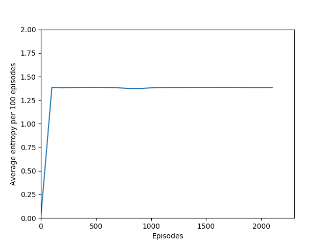
A minor training issue I encountered: since the outputs of the policy logits are at first very similar, putting them through a softmax distribution and then sampling from it meant that the agent was following a more or less random policy, which made it impossible to learn from experience — any tiny changes to the network weights would just be drowned out by the random sampling. A probability distribution of 0.25/0.25/0.25/0.25 is not a whole lot different than 0.245/0.247/0.253/0.255 when you’re sampling from it. I also discovered that adding noise to the outputs to encourage exploration simply meant that the agent had a harder time following its policy, and that the noise again drowned out the changes in the policy in the early episodes of learning, which are critical to bootstrapping. Taking the argmax of the outputted action probabilites was the way to go, since it offered the most consistency with the actor’s behavior and the network’s outputs — argmax is very sensitive to small changes when all the probabilities are very similar.

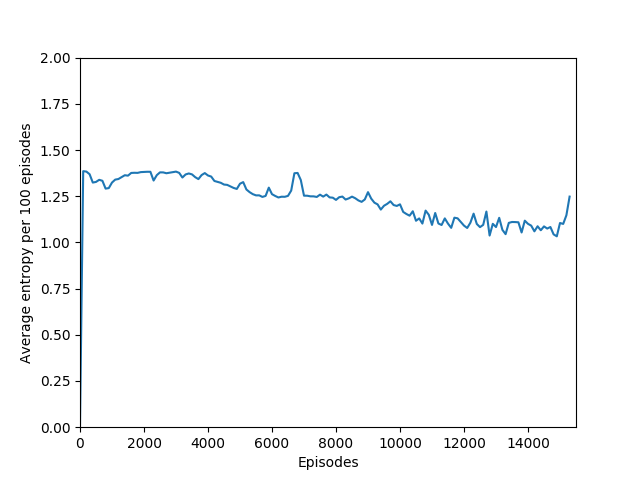
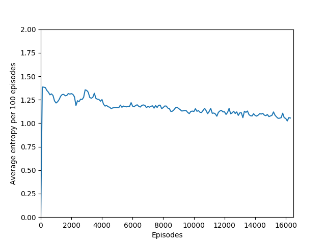
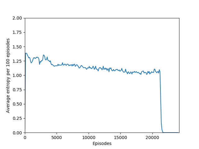
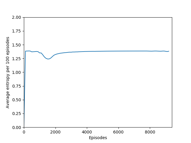
Note that 1.38, the value at the flat line in the graph, is the entropy for the probability distribution 0.25/0.25/0.25/0.25.

This also had to do with the fact that our total loss, used to optimize both the actor and the critic, combined the actor loss, the critic loss, and a negative entropy term, which actually had the effect of pushing the policy action probabilites closer to a random policy: minimizing negative entropy means maximizing entropy, leading the network to be more “uncertain” about which action to take. While this may sound like a bad idea, it is actually necessary to prevent the algorithm from falling into some very easy local minima right off the bat by taking the same action to the exclusion of all others, making it impossible to learn anything but that suboptimal behavior. For example, training without the entropy term or with the entropy term’s sign flipped made the agent in Breakout move the paddle all the way to the right and do nothing but try to move the paddle right.

Finally, after correcting that big misunderstanding, I found some sort of learning rate decay necessary in order to skirt the local minima of the objective function in the early stages of training. If we kept the learning rate constant, the network would learn to hit the ball once or twice, perhaps even getting up to 30 reward or so, and then unlearn all of it and just move the paddle right. However, learning rate decay allows the network to value later learning less than initial learning, which makes sense since games of Breakout all look about the same at the beginning and we want to quickly learn the behavior of hitting the ball, but as the games progress, they tend to look different and we want to learn just enough that the agent can hit the ball but not too much that it thinks that some configuration of the blocks means that it should arbitrarily move left or right. Decaying the learning rate allows us to initially take large steps to step over early local minima and smaller steps later on once the algorithm is close to the true minimum.

I used a simple linear learning rate decay policy where the initial learning rate was decayed linearly over several million training iterations, but I wonder if different decay strategies like quadratic or exponential might make a difference in avoiding the sharp overfitting dropoff that we can see towards the end of training.

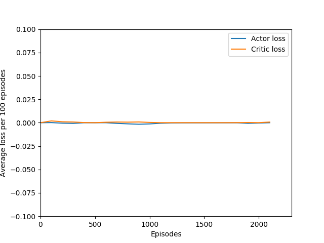
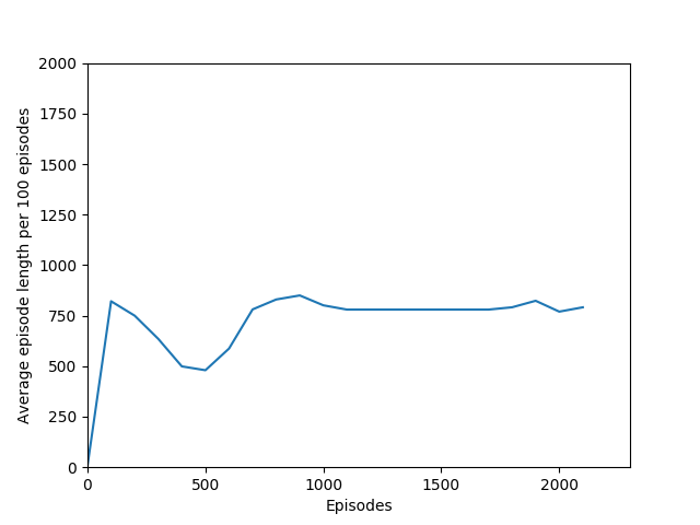
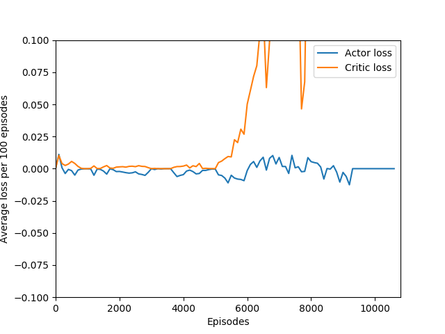
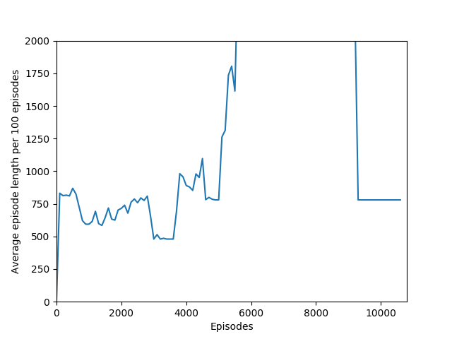
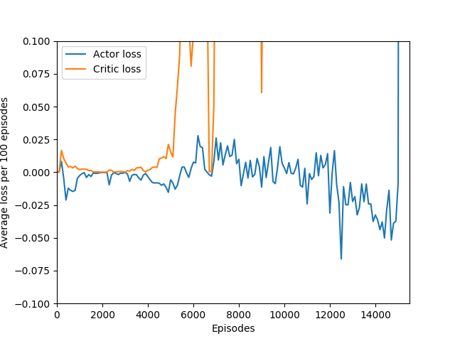
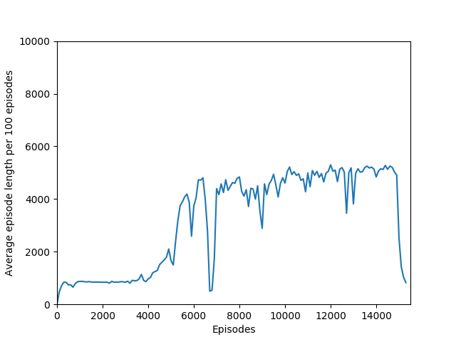
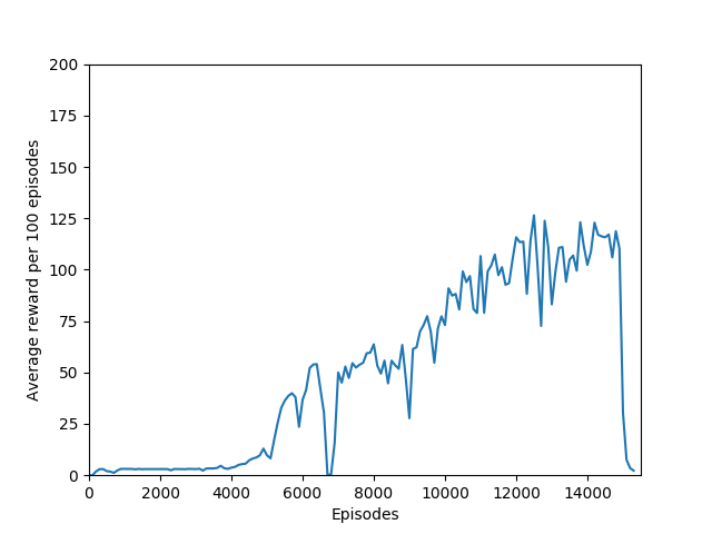
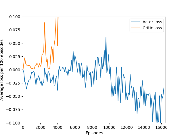
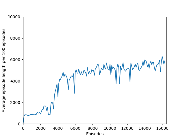
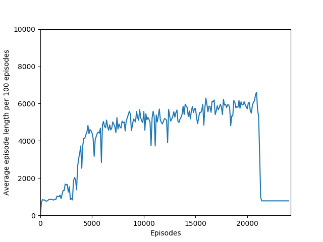
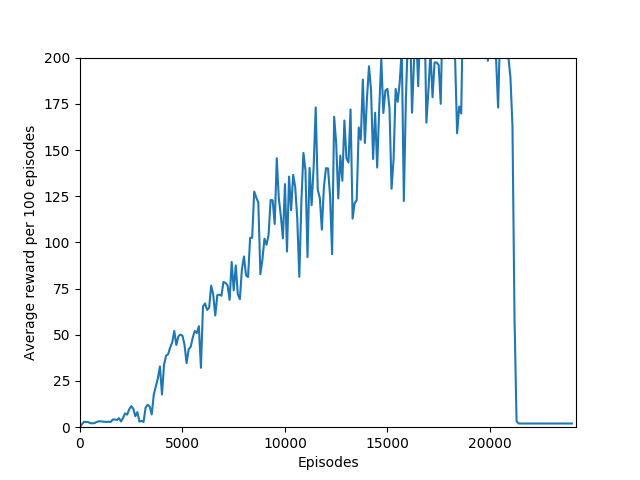
Some comments on the generated graphs: because we are slightly pushing entropy to be high in the loss function to avoid the network prematurely preferring one action to the exclusion of all others, the entropy should remain fairly high and fairly constant, but it should certainly not flatline as 1.38, which is the value associated with a random policy. It is interesting to see how the losses are related to the episode length and the average reward, and episode length and rewards are very closely correlated, since games of Breakout lasting longer = a higher score. Also note that I am averaging rewards per episode over 100 episodes, which trades precision for a better look at the overall trend of learning – the reward gotten per episode usually has quite a high variance, so a higher average reward per 100 episodes really means that it is consistently getting better. A more precise graph would probably use average reward per 20 or 25 episodes.

Apologies for some of the graphs running over their axes — I have so far only run on my local machine but plan to run on cloud compute next.

N = 5

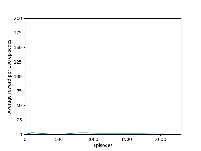
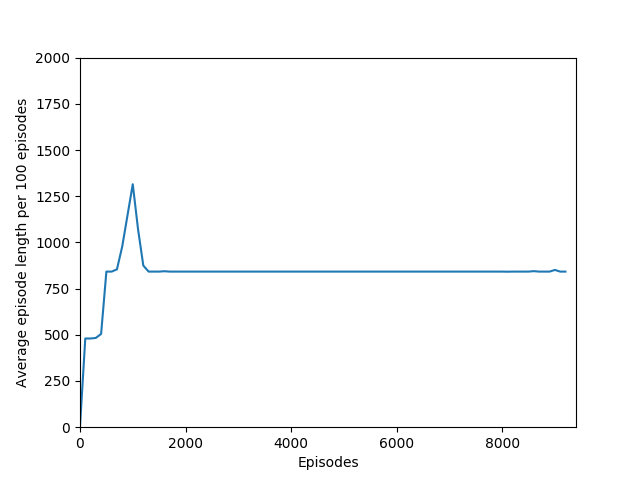
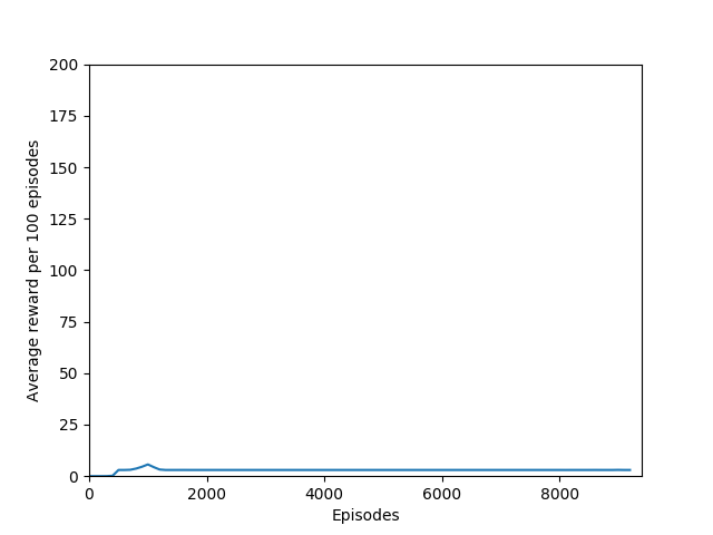
I have not yet run the N = 5 case extensively, but in the 3000 or so episodes I did run it, it did not seem to learn anything. More details (# iterations, etc.) to come as I train this for longer. For now, these graphs provide a good look at what an agent that doesn’t learn anything looks like.

N = 20

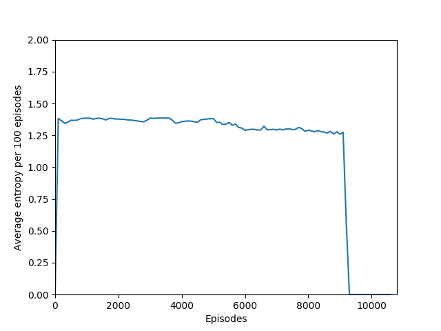
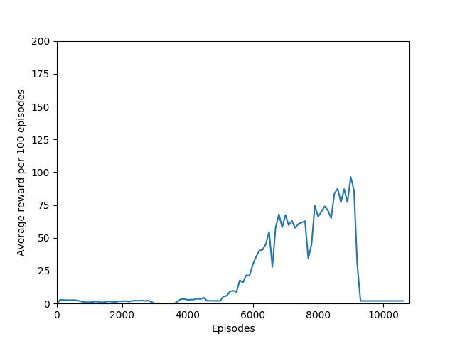
N = 20 was the first case to show promising results — it was able to get up to a max reward of 376 and a good average reward per 100 episodes, although it wasn’t quite able to get over 200 average reward per 100 episodes before the overfitting cliff hit, which was at around 9000 training episodes (4M iterations).

N = 50

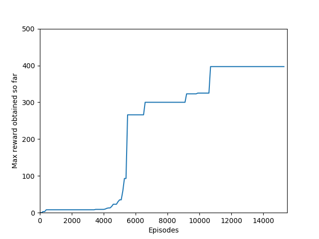
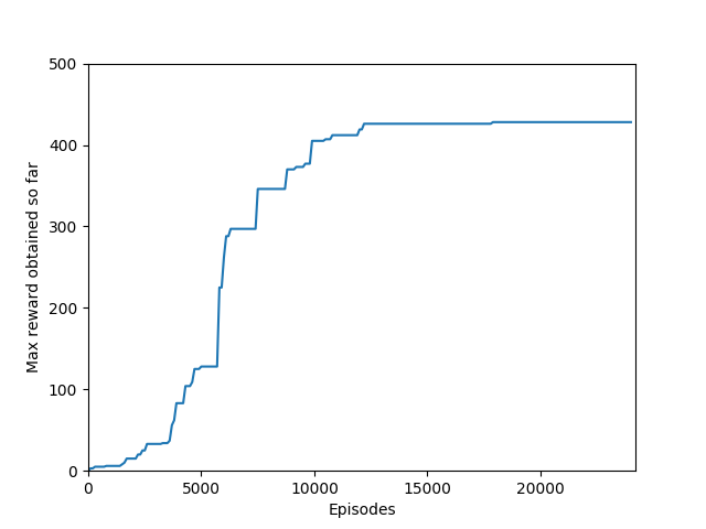
N = 50 performed even better than N = 20, and since I began graphing the max reward obtained so far, N = 50 was able to get a somewhat but not significantly higher max reward of 397, though it took significantly longer to train (in terms of # of episodes, not sure yet about # iterations). N = 50 also had a policy that appeared more stable, likely because unrolling over more time steps trades training speed and immediate reward for a more long-term outlook both in the agent and in training.

N = 100

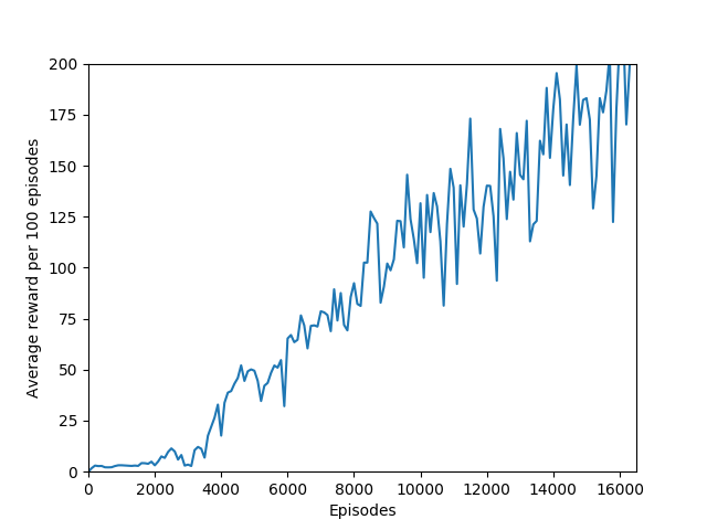
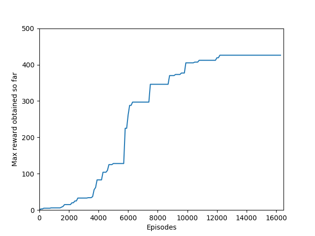
N = 100 was the slowest training agent that I had run so far, but it certainly did a good job of learning how to play Breakout, likely because 100 is a particuarly good number of steps, about the number of steps that it takes for the paddle to hit the ball and for the ball to hit the bricks and reward to be issued, which makes it particularly good for a rollout as each batch of 100 steps would include the paddle actually hitting the ball as well as the reward being issued. The max reward achieved is 428 and average reward per 100 episodes exceeded 200 towards the end of training.

At around 10400 episodes of training, the agent exhibits the advanced behavior of focusing hitting the ball towards one side of the wall, thus making a tunnel to hit the ball through and score a huge reward when the ball repeatedly bounces off the far wall and the higher-valued bricks in the back.

Here are two video captures from 11400 and 11900 episodes of training where it digs a tunnel through the center as well as a tunnel through the side and even catches the ball when it comes out one of the side tunnels, even though it was hit through the center tunnel.

Finally, here are two video captures from 15500 and 17800 training episodes where the agent has more or less solved the game, hitting almost every brick on the screen.

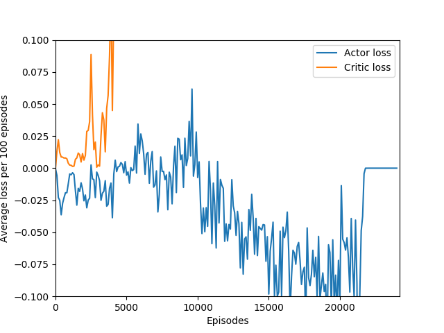
Unfortunately, after a week of training on my laptop, this model too hit the overfitting cliff. Here are the graphs from the end of training:

And here’s a video of the final policy. Note that it does seem to have retained something, but the policy logits are outputting action-probabilities that have the 1 on the move right action, which is usually what these learning algorithms resort to in this game when there’s a bug in the code or if they are not complex enough to learn how to play the game.

N = infinity

I found that N = infinity was not able to learn anything, most likely because the unrolling takes place over several hundred time steps and the rewards just become too diluted to train worth anything. Also, if the only estimated state-value wrapped into the rollout is that of the terminal state, then it removes the effect of even having a critic — the critic estimate is always disregarded in training and the estimated state-value is discarded. Even if it were run for a very long time, I doubt that it would be able to learn Breakout.

Reflection

There is also the very interesting steep dropoff towards the end of training when the agent seems to suddenly stop being able to play breakout. From video capture, it seems as if the agent can still move the paddle to more or less the right place but can’t keep it there to hit the ball, instead moving it aside at the last moment. This likely starts a positive feedback loop, resulting in the agent repeatedly achieving very little reward with the weights that it learned, leading to it unlearning how to play breakout in a cascade of poor episodes caused by just missing the ball.

And eventually, it performs more or less like a random agent.

Here is a video capture of a lucky random policy, for comparison:

In any case, my agent was able to achieve consistently 200+ reward, which is considered to have “solved” Breakout. Certainly it matches, if not surpasses, human-level performance, and besides the fact that a critical misunderstanding in the A2C algorithm took me two months to unravel, this was an extremely informative learning experience. Writing the code for the algorithm and the network was the easy part. The hard part was training and debugging. I was lucky in that respect — I found an implementation of the algorithm worked that I could look at to see which features it had that my code didn’t, and then implement them in my own code one by one.

Some very interesting questions that I would like to explore: why do smaller values of N even work, considering that the action that resulted in the paddle hitting the ball and the reward being issued may not even take place in the same N time steps? Particularly for N = 20 — how was it able to learn something when the reward definitely was not issued in the same batch as the action that led to the reward? Exactly how much of a role does entropy and the critic loss play — I used the canned coefficients of 0.5 for the critic loss and 0.1 for the entropy, but would the agent learn faster if the critic loss coefficient was increased, placing relatively more value on the quality of the network’s estimates, or if the entropy coefficient was increased (encouraging more evenly-distributed action probabilities) or decreased (encouraging more confident, distinct action probabilities).

And the biggest question of all: what exactly is the cliff at the end of training? I have observed that the cliff happens when the softmax action probabilities converge to all zeroes and one one. It must be some sort of overfitting, but is it in the same vein as overfitting in supervised learning, or is it something different? It is a very sharp drop rather than a slow decline, which means that the agent was very good at playing the game before somewhat suddenly becoming very bad. Breakout is deterministic, which means that the loss of uncertainty whould be a good sign — likely, the wrong kernels/units are being overly emphasized, which leads to worse decisions.

An interesting hint is that the actor loss goes to zero (again, because probability of choosing the action that it chose becomes 1 and the log of that becomes 0) but the critic loss explodes, becoming something around 10+ digits long, which hints us that the value estimate for each state is exploding while the obtained rewards stagnate or drop sharply, and since the critic loss is the difference of the two squared, it results in an extremely large loss, which is likely the reason for the agent’s quick decline in performance. This seems quite like a case of exploding gradients, where the network’s state-value estimate goes to infinity or negative infinity (likely the latter) and causes a positive feedback loop where the loss gets larger and larger and the gradients get larger and larger.

All in all, a very very good learning experience. Who knew that reinforcement learning was so hard? :P